Problem Set 1 Diffusion
Goals: approximation, standard curve, scale, spreadsheet best practices, google search
The main goal of this exercise is to use approximation to demonstrate that diffusion is too “slow” to be an effective transport process at any scale larger than microscopic (microns). Scale roughly means size but typically size means something fairly precise (132.5 cm) while scale is more general. “At the scale of individual molecules” means something with a size of 1 nm or 10 nm or even 100 nm but certainly no 10^5 nm. When using scale, our precision is generally only at the order of magnitude, which are multiples of 10 (The range 1 nm to 100 nm is over two orders of magntidue).
1.1 Approximation
At some point, scientists are confronted with the recognition that some math problems do not have exact answers. This is very different than the math we learn in high school and college, which typically represents math as a construction that only has exact answers (2 + 2 = 4 and not any other number).
What is the expected time of diffusion of biologically important molecules at different scales? There is no exact answer to a question like “how long does it take for oxygen to diffuse across the respiratory membrane”. Instead there are better answers and worse answers. The reason there isn’t an exact answer is because
- the question is about a system of particles that are in diffusion. The motion of individual particles is random and the time an individual particle travels a certain net distance is a function of its individual history of elastic collisions with other particles. But we can compute expected (or the average) time for diffusion over a specified distance using a simple diffusion model (see below)
- The rate of diffusion is a function of the medium such as pure water, air, cytosol, or lipid bilayer. The diffusion coefficient in the table below is measured using water as the medium but in the questions below the media might include cytosol, extracellular fluid, and phospholipid membrane, so the water-based coefficient will only give us a close (or approximate) answer.
- The final reason is the one that makes students the most uncomfortable. The goal of this exercise is to compare time of transport by diffusion over distances that differ by many orders of magnitude–from a few nm to a few meters (so one billion times or 9 orders of magnitude). While it is true that skeletal muscle cells vary in diameter and the epidermis varies in thickness, the question is looking for a answer only at a reasonable order of magnitude. Two meters is a reasonable answer to the question, what is the height of humans? 0.2 or 20 meters is not.
1.2 Problems
A simple formula to calculate the approximate time of diffusion (t) over a distance (x) is
\[\begin{equation} t \approx \frac{x^2}{2D} \end{equation}\]where D is a diffusion coefficient. The symbol \(\approx\) means “approximately equal to”.
1.2.1 Compute diffusion times for chemicals with known diffusion coefficients
Create a table in your sheet that looks like this:
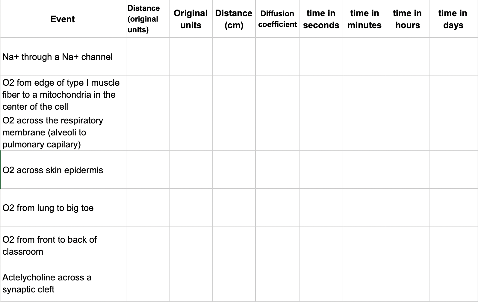
The first column lists diffusion “events”, for example, the diffusion of a sodium ion (Na\(^+\)) through a Na\(^+\) channel. Use Google search to find the distance traveled by the chemical in each event. Use this distance, the molecular weight of the molecule (see the table below), and the function above to compute the approximate time for transport of this molecule across this distance via diffusion. Compute this time in seconds, minutes, hours, and days. See Problem 2 below for actylcholine.
Spreadsheet best practices that must be followed to receive full points;
Use functions for all math; that is, don’t do the math in your head or on a calculator and input the result. Do the math in the spreadsheet. The reason for doing the math in this worksheet is that this is good practice. If we do math on a calculator and then insert the result here, we have no record of the computation. Having a record of all computations is a best practice for reproducible science.
Keep cells with numeric values (such as the diffusion distance) numeric. For example, do not add units to the diffusion distance in the cell containing the numeric value. If the diffusion distance is 1 meter, enter “1” into the cell and not “1 meter”. The reason is, you can’t do math on words (that is, the value in the cell won’t work in simple equations). But, it is good to record the units so add these to the adjacent column (Original units).
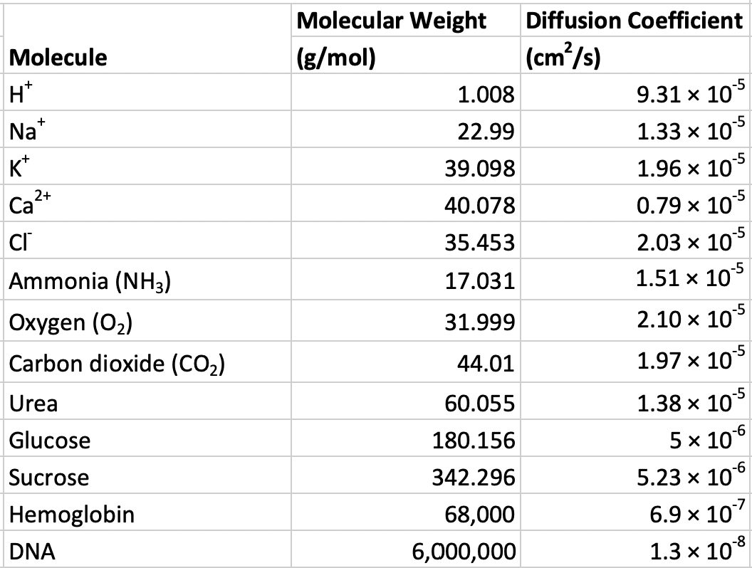
Figure 1.1: Molecular weights of common biological molecules
1.2.2 Compute diffusion time for a chemical with an unknown diffusion coefficient
Diffusion data for acetylcholine is not given in the table above. You might be able to find the coefficient with a google search but I want you to use the table of above to 1) generate a standard curve and 2) use the generated curve to estimate the diffusion coefficient for acetylcholine. Remember that diffusion is a function of the size of the molecule – bigger molecules diffuse more slowly. In other words, the diffusion coefficient gets smaller as the size of the molecule gets bigger. Use the table above to create a standard curve, which shows the relationship between known X and known Y. Standard curves are everywhere in science research and recognizing that you can solve a problem, without asking for help, by generating a standard curve will make your future boss very happy. So, instead of trying to look up the diffusion coefficient of acetylcholine, look up its molecular weight with a quick google search (or test your chemical skills and compute its weight using acetylcholine’s chemical formula) and compute its expected (or predicted value) given the standard curve.
In a traditional standard curve done on graph paper, one can predict the expected value of Y (which has not been directly measured) from the known value of X. Here, I want you to do this by generating the mapping function (a function that maps a value of X to a value of Y)
\[\begin{equation} D = b_0 + b_1 MW \end{equation}\]which is the equation for a line (recognize how it is simply Y = mX + b with b and mX re-arranged?) so \(b_0\) is the intercept and \(b_1\) is the slope. Use the data in the table to estimate the slope and intercept of the mapping function and then use this slope and intercept to compute the estimated diffusion coefficient for acetylcholine. When computing the slope and intercept, temember that we want to predict D from MW.
- log transform the weights and the diffusion coefficients– this will make the relationship between the two linear.
- plot log(D) on the Y-axis aganst log(MW) on the X-axis. Show the “trend line”, also called the regression line and formula, which gives the slope and intercept
- In seperate cells, use spreadsheet functions (google these) to compute the slope and intercept
- use the equation for the regression line to compute the predicted log(diffusion coefficient) given a the log(molecular weight of acetylcholine). Use the cells with the slope and intercept in this function. ** Do not hardcode the slope and intercept in your formula **.
- back transform the answer to get the right units (not log units) - the back-transformation is the inverse or anti-log. Make sure you know the base for the log function that you are using!