Chapter 7 Creating Fake Data
Fake data are generated by sampling from one of R’s random sampling functions. These functions sample from different distributions including
- uniform – function
runif(n, min=0, max=1), which samples n continous values betweenminandmax. - normal (Gaussian) – function
rnorm(n, mean=0, sd=1), which samples n continous values from a distribution with the specified mean and standard deviation. The default is the “standard” normal distribution. - poisson – function
rpois(n, lambda), which samplesncounts from a distribution with mean and variance equal tolambda. - negative binomial –
rnegbin(n, mu=n, theta), which samplesncounts with meanmuand variancemu + mu^2/theta.
7.0.1 Continuous X (fake observational data)
A very simple simulation of observational design (the are not at “controlled” levels)
n <- 25
# the paramters
beta_0 <- 25 # the true intercept
beta_1 <- 3.4 # the true slope
sigma <- 2 # the true standard deviation

x <- rnorm(n)
y <- beta_0 + beta_1*x + rnorm(n, sd=sigma)
qplot(x, y)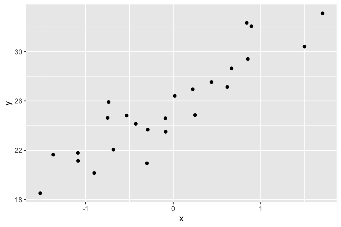
How well does a model fit to the data recover the true parameters?
| Estimate | Std. Error | t value | Pr(>|t|) | |
|---|---|---|---|---|
| (Intercept) | 25.8 | 0.34 | 75.8 | 0 |
| x | 4.2 | 0.40 | 10.4 | 0 |
The coefficient of is the “Estimate”. How close is the estimate? Run the simulation several times to look at the variation in the estimate – this will give you a sense of the uncertainty. Increase and explore this uncertainty. Increase all the way up to . Commenting out the qplot line will make this exploration easier.
7.0.2 Categorical X (fake experimental data)
Similar to above but the are at controlled levels and so this simulates an experimental design
n <- 5 # the sample size per treatment level

fake_data <- data.table(Treatment=rep(c("control", "treated"), each=n))
beta_0 <- 10.5 # mean of untreated
beta_1 <- 2.1 # difference in means (treated - untreated)
sigma <- 3 # the error standard deviation
# the Y variable ("Response") is a function of treatment. We use some matrix
# algebra to get this done.
# Turn the Treatment assignment into a model matrix. Take a peak at X!
X <- model.matrix(~ Treatment, fake_data)
# to make the math easier the coefficients are collected into a vector
beta <- c(beta_0, beta_1)
# you will see the formula Y=Xb many times. Here it is coded in R
fake_data[, Response:=X%*%beta + rnorm(n, sd=sigma)]
# plot it with a strip chart (often called a "dot plot")
ggstripchart(data=fake_data, x="Treatment", y="Response", add = c("mean_se"))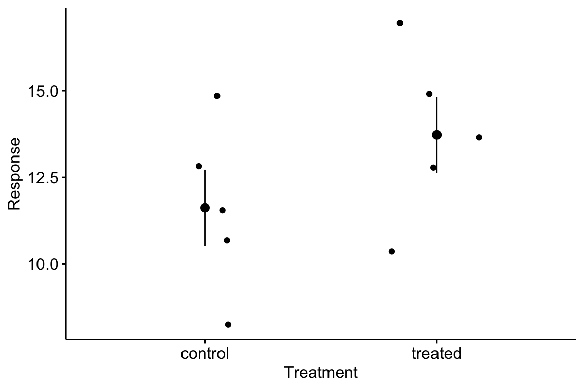
# fit using base R linear model function
fit <- lm(Response ~ Treatment, data=fake_data)
# display a pretty table of the coefficients
knitr::kable(coefficients(summary(fit)), digits=3)| Estimate | Std. Error | t value | Pr(>|t|) | |
|---|---|---|---|---|
| (Intercept) | 11.626 | 1.097 | 10.601 | 0.000 |
| Treatmenttreated | 2.100 | 1.551 | 1.354 | 0.213 |
Check that the intercept is close to beta_0 and the coefficient for Treatment is close to beta_1. This coefficient is the difference in means between the treatment levels. It is the simulated effect. Again, change . Good values are and . Again, comment out the plot line to make exploration more efficient.
7.0.3 Correlated X (fake observational data)
7.0.3.1 Generating correlated X variables
It’s useful to think about how correlated data are generated because often we want to generate fake_data with an expected correlation. Let’s say we want to generate two X variables that have an expected correlation of 0.6. To generate this, we take advantage of the fact that two variables, X1 and X2, are correlated if they share a “common cause” – a variable Z that effects (or “causes”) both X1 and X2. If the expected variances of X1, X2, and Z are all 1, then the expected correlation between X1 and X2 is the product of the causal effect from Z to each X. The easiest way to implement this is to simply make the effect from Z to both X equal to .
n <- 10^3
z <- rnorm(n) # the common cause, with sigma = 1
rho <- 0.6 # the true correlation between X1 and X2
beta_z <- sqrt(rho) # the easiest way to get effects of z on X1 and X2 that generates rho
sigma_x <- sqrt(1 - rho) # we will make the variance of X1 and X2 = 1, so the "explained" variance in X is beta_z^2 = rho so this is the sqrt of the unexplained variance
x1 <- beta_z*z + rnorm(n, sd=sigma_x)
x2 <- beta_z*z + rnorm(n, sd=sigma_x)
# check
cov(data.frame(X1=x1, X2=x2)) # is the diagonal close to 1, 1?
## X1 X2
## X1 1.0523598 0.5978408
## X2 0.5978408 0.9713292## [1] 0.5913168
Now create fake that is a function of both and . Create “standardized” fake data, where .
beta_0 <- 3.2
beta_1 <- 0.7
beta_2 <- -0.3
explained_sigma <- beta_1^2 + beta_2^2 + 2*beta_1*beta_2*rho # Wright's rules! Compare to Trig!
sigma_Y.X <- sqrt(1 - explained_sigma) # sqrt unexplained variance
y <- beta_0 + beta_1*x1 + beta_2*x2 + rnorm(n, sd=sigma_Y.X)

# check
var(y) # should be close to 1 as n gets bigger
## [1] 0.9791502## Estimate Std. Error t value Pr(>|t|)
## (Intercept) 3.1887712 0.02536483 125.716255 0.000000e+00
## x1 0.6885565 0.03064195 22.471043 8.422461e-91
## x2 -0.3037457 0.03189446 -9.523465 1.223898e-20Note that the variance of is the variance of the explained part due to X1 and X2 and the unexplained part and if the expected variance of then this sets an upper limit for the explained part. This means that
which means the magnitude of and should generally be less than 1.
7.0.3.2 Creating mulitple X variables using the package mvtnorm
The package mvtnorm provides a function to generate multivariate data (multiple columns) with a specified vector of means (the means of each column) and covariance matrix among the means.
rcov1 <- function(p){
  # p is the number of columns or number of variables
  pp <- p*(p-1)/2 # number of elements in lower tri
  max_r <- 0.7
  r <- rexp(pp)
  r <- r*max_r/max(r)

  # create correlation matrix
  R <- matrix(1, nrow=p, ncol=p)
  R[lower.tri(R, diag=FALSE)] <- r
  R <- t(R)
  R[lower.tri(R, diag=FALSE)] <- r

  # convert to covariance matrix
  L <- diag(sqrt(rexp(p))) # standard deviations
  S <- L%*%R%*%L

  # check -- these should be the same
  # R
  # cov2cor(S)
  return(S)
}
Now let’s use mvtnorm to generate fake correlated X
p <- 5 # number of X variables
S <- rcov1(p)

# make the fake X
n <- 10^5
mu <- runif(p, min=10, max=100) # vecctor of p means
X <- rmvnorm(n, mean=mu, sigma=S)

# how close? (check the cor as this is easier to scan)
cov2cor(S)
## [,1] [,2] [,3] [,4] [,5]
## [1,] 1.0000000 0.15511020 0.11863165 0.48788949 0.14545246
## [2,] 0.1551102 1.00000000 0.70000000 0.03514487 0.04345391
## [3,] 0.1186317 0.70000000 1.00000000 0.05346376 0.54083807
## [4,] 0.4878895 0.03514487 0.05346376 1.00000000 0.44504979
## [5,] 0.1454525 0.04345391 0.54083807 0.44504979 1.00000000## [,1] [,2] [,3] [,4] [,5]
## [1,] 1.0000000 0.15618693 0.12146387 0.48987841 0.14569745
## [2,] 0.1561869 1.00000000 0.69709529 0.03879653 0.03961509
## [3,] 0.1214639 0.69709529 1.00000000 0.05598629 0.54138395
## [4,] 0.4898784 0.03879653 0.05598629 1.00000000 0.44214983
## [5,] 0.1456974 0.03961509 0.54138395 0.44214983 1.000000007.0.3.3 The rcov1 algorithm is naive
A problem with generating a fake covariance matrix as above is that it is likely to be singular as get’s bigger. A singular covariance matrix is one where there are fewer orthogonal axes of variation then there are variables. Imagine a multidimensional scatterplot of a data set with the fake covariance matrix. If we zoom around this multidimensional space, we will come across a “view” in which all the points are compressed along a single line – that is there is no variation on the axis orthogonal to this line of points. This is bad, as it means we cannot fit a linear model using least squares (because the inverse of the covariance matrix doesn’t exist).
Let’s explore this. If the a covariance matrix is singular, then at least one eigenvalue of the matrix is negative (eigenvalues is a multivariate term beyond the scope of this text but, effectively, these are the variances of the orthogonal axes referred to above). Here I compute the frequency of covariance matrices with at least one negative eigenvalue as increases
niter <- 1000
p_vec <- 3:10
counts <- numeric(length(p_vec))
i <- 0
for(p in 3:10){
  i <- i+1
  for(iter in 1:niter){
    counts[i] <- ifelse(eigen(rcov1(p))$values[p] < 0, counts[i]+1, counts[i])
  }
}
data.table(p=p_vec, freq=counts/niter)
## p freq
## 1: 3 0.000
## 2: 4 0.025
## 3: 5 0.066
## 4: 6 0.135
## 5: 7 0.190
## 6: 8 0.225
## 7: 9 0.275
## 8: 10 0.3687.0.3.4 Generating multiple columns of X variables with a non-singular covariance matrix
This section uses some ideas from matrix algebra. The goal is to create a matrix of variables that have some random covariance structure that is full-rank (not singular, or no negative eigenvalues). The algorithm starts with a random eigenvector matrix and a random eigenvalue matrix and then computes the random covariance matrix using
- Generate a random random eigenvector matrix from a covariance matrix of matrix of random normal variables.
fake.eigenvectors <- function(p){
    a <- matrix(rnorm(p*p), p, p) # only orthogonal if p is infinity so need to orthogonalize it
    a <- t(a)%*%a # this is the sum-of-squares-and-cross-product-matrix
    E <- eigen(a)$vectors # decompose to truly orthogonal columns
    return(E)
}- Generate random eigenvalues in descending order and that sum to 1. There are several ways to create this sequence. Here are two:
# force the eigenvalues to descend at a constant rate
fake.eigenvalues <- function(p, m=p, start=1, rate=1){
  # m is the number of positive eigenvalues
  # start and rate control the decline in the eigenvalue
  s <- start/seq(1:m)^rate
  s <- c(s, rep(0, p-m)) # add zero eigenvalues
  L <- diag(s/sum(s)*m) # rescale so that sum(s)=m and put into matrix,
  # which would occur if all the traits are variance standardized
  return(L)
}

# random descent
fake.eigenvalues.exp <- function(p, m=p, rate=1){
  # exponential distribution of eigenvalues
  # m is the number of positive eigenvalues
  # start and rate control the decline in the eigenvalue
  s <- rexp(m, rate)
  s <- s[order(s, decreasing=TRUE)] # re-order into descending order
  s <- c(s, rep(0, p-m)) # add zero eigenvalues
  L <- diag(s/sum(s)*m) # rescale so that sum(s)=m and put into matrix,
  # which would occur if all the traits are variance standardized
  return(L)
}- Generate the random covariance matrix
fake.cov.matrix <- function(p){
    # p is the size of the matrix (number of cols and rows)
    E <- fake.eigenvectors(p)
    L <- diag(fake.eigenvalues(p))
    S <- E%*%L%*%t(E)
    return(S)
}- Generate the random variables using
# two functions to compute the random data
fake.X <- function(n,p,E,L){
  # n is number of observations
  # p is number of variables
  X <- matrix(rnorm(n*p),nrow=n,ncol=p) %*% t(E%*%sqrt(L))
    return(X)
}
An example
n <- 10^5
p <- 5
E <- fake.eigenvectors(p)
L <- fake.eigenvalues(p, start=1, rate=1)
X <- fake.X(n, p, E, L)
colnames(X) <- paste0("X", 1:p)
E
## [,1] [,2] [,3] [,4] [,5]
## [1,] 0.4762049 0.76679336 0.02189702 -0.37886958 -0.20306443
## [2,] -0.3226816 0.26514622 -0.21147219 0.50680583 -0.72387940
## [3,] 0.6343127 -0.07414265 0.40381446 0.65434666 0.03024185
## [4,] 0.2450305 -0.53523178 0.22900376 -0.40906173 -0.65856872
## [5,] -0.4546568 0.22305882 0.85982044 -0.06406746 -0.01166667E <- eigen(cov(X))$vectors
scores <- X%*%E
colnames(scores) <- paste0("pc", 1:p)
cor(cbind(X, scores))[1:p, (p+1):(p*2)]## pc1 pc2 pc3 pc4 pc5
## X1 0.6381822 0.71536319 0.009665104 0.2581645 -0.119317350
## X2 -0.5701649 0.32632936 -0.213505507 -0.4289443 -0.582102493
## X3 0.8417769 -0.06005797 0.312645510 -0.4358132 0.011149679
## X4 0.4130194 -0.64271492 0.232581875 0.3517727 -0.488358607
## X5 -0.6579685 0.23893819 0.712352851 0.0501983 -0.004418134