Chapter 6 An Introduction to Statistical Modeling
6.1 This text is about the estimation of treatment effects and the uncertainty in our estimates. This, raises the question, what is “an effect”?
Chapter 1 introduced a completed R Markdown document for a set of experiments on the consequences of deletion of the ASK1 signaling protein on diet-induced obesity and glucose and fat metabolism in mice. Let’s think about the goal of the statistical analyses of these data, using the experiment in Figure 2e as our focus.
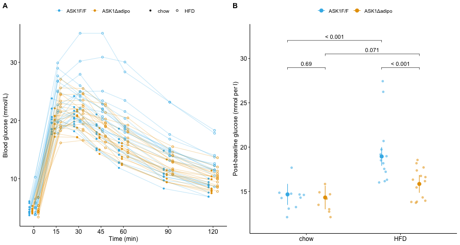
Figure 6.1: A. Blood glucose levels at each time point in each mouse. B. Average post-baseline blood glucose adjusted for baseline value. Unadjusted p-values are from the model mean_glucose ~ baseline + ask1 + diet + ask1:diet.
After a meal rich in glucose, blood glucose levels rise from their fasting level to a peak as glucose is transported from the intestine into the blood. The hormone insulin signals muscle and adipose cells to take up this glucose. The consequence of this transport is, over a period of about two hours, blood glucose levels return to fasting levels. In the experiment for Figure 2e, instead of introducing glucose through the mouth, the researchers injected glucose into the peritoneal cavity, which surrounds the organs of the abdomen. From the peritoneal cavity, glucose diffused into the blood. Blood glucose levels were measured immediately prior to the peritoneal injection, and 15, 30, 45, 60, 90, and 120 minutes after injection. The initial, pre-injection measure is the baseline measure. My version of the glucose level at these time points is shown above in Figure 6.1A.
The researchers used this experiment to explore the consequence of ASK1 knockout on glucose tolerance – a high initial maximum and a slow decline are indicators of glucose intolerance. A researcher could compare many features of the glucose curves in Figure 6.1A, including the magnitude of the initial maximum or the rate of decline. The researchers used the area under the curve(AUC) for each mouse as a summary measure of glucose processing. A better measure would be the AUC of only the post-baseline time points, because (1) only the post-baseline values reflect the differential response to blood glucose and (2) comparing post-baseline values avoids a phenomenon called regression to the mean, which is covered in the chapter on “Adding covariates to a linear model”. And, because AUC is in units (mmol/L minutes) that aren’t especially meaningful, a better measure is the average glucose level over the post-baseline time period, which is computed as the post-baseline AUC divided by the post-baseline duration (115 minutes).
Some questions a researcher might be interested in with this experiment are
When on a high fat diet, does knocking out ASK1 improve glucose tolerance relative to functional ASK1? If there really is an improvement in glucose tolerance in the ASK1 knockout, then we expect the mean post-baseline level of the ASK1 mice to be smaller than the mean post-baseline level of the control mice. That is, we expect a difference in means. A difference in the response of a variable to a treatment is called an effect. At this level of inquiry, a researcher is asking only does an effect exist, and what is the sign (does ASK1 knockout improve or decrease glucose tolerance?) and not the magnitude of the effect (does ASK1 knock improve glucose tolerance greatly, moderately or trivially?). For this kind of question, we can use a signficiance test, which generates a test-statistic and a p-value. This kind of query is the minimal level of knowledge for understanding a system. It can be used to identifying the agents in a system but not much about the dynamics of the system.
When on a high fat diet, how much does the knockout of ASK1 improve glucose tolerance, relative to mice with functional ASK1? For this kind of question, we want to estimate the true effect (that is, estimate its magnitude and sign) and we want a measure of our uncertainty in this estimate. A standard error of the difference in means is a measure of the precision of our estimate and can be used to compute a confidence interval of the difference in means, which is a measure of uncertainty. With an estimate of the magnitude of the true effect, a researcher can begin to compare the importance of different agents in a system, to know which might be the targets of intervention, for example. In a heavily competitive grant environment, demonstrating that the focus of the research (ASK1) not only has an effect, but has a large effect (relative to other potential agents), should be an important consideration for any funding decision.
When on a high fat diet, what is the dose-response relationship between ASK1 activity level (how much is active?) and the rate of glucose clearance? In a real system, the level of a signaling molecule like ASK1 in a cell is not “all or none” but is continuous, from something low to something high. To understand the dynamics of ASK1 within the larger signaling system controlling browning of white adipose tissue cells, researchers need to know the expected blood glucose conditional on the concentration of ASK1. For this kind of query, a researcher fits a curve (potentially non-linear) and the slope of the curve at any level of ASK1 is the effect. The effect is the difference in mean glucose per unit difference in ASK1. Reserchers can use these effect estimates as parameters in quantitative models of a system in order to predict how a system behaves given different kinds of interventions.
Inquiry level 3 requires a specific kind of experimental design (what is called a regression design), so needs to be planned in advance. Inquiry level 2 is strongly advocated in this text and elsewhere because it addresses why we should care about a result – is this difference important in the system and worth the time and money in this lab, or is it trivial and should be discarded in favor of pursuing more important agents in this system? Almost all research in experimental biology communicates results at inquiry level 1 only, but a researcher can always add estimates of treatment effects and the uncertainty in these estimates. For some experiments, estimates of the magnitude of an effect are not very meaningful or useful because the response variable is measured with a tool that doesn’t have very meaningful units (for example “intensity” of a scanned gel). Ideally, these non-meaningful units can be turned into something meaningful (amount of protein). If they cannot (or are not), then inquiry level 1 is an appropriate level for communication of the result.
A summary of this:
- Inquiry level 1: Is there an effect? If so, what is the direction? – this is the classic hypothesis testing strategy
- Inquiry level 2: How big is the effect? Is it big enough to want to study it? – this requires additional analysis than level 1, the estimation of effects and of the uncertainty in the effect.
- Inquiry level 3: How does the response change with incremental change in the treatment? – this is analyzed as in level 2 but also requires a regression design.
This book is about the estimation of effects of experimental treatments using linear models. It may seem strange to have to use a linear model to estimate an effect – if an effect is a difference in means, why not just compute the means and the difference in means using elementary school math and call it a day. My answer has two parts
- With simple experimental designs, a researcher can estimate the effect by simply computing the difference between two means. But there’s not much a researcher can do with this number. In order to move forward with any kind of inference, such as estimating the standard errors of the means, or of computing p-values, a researcher needs a statistical model.
- In anything other than the simple experimental designs, an effect computed from the raw means between treatment groups can give a less precise or even a misleading estimate of the estimate. Instead of raw means, what we need are conditional means estimated from a statistical model. An example is the means of the groups in Figure 6.1B, which are adjusted for the baseline glucose values.
6.2 An introduction to linear models
This chapter introduces statistical modeling using the linear model. All students are familiar with the idea of a linear model from learning the equation of a line, which is
\[\begin{equation} Y = mX + b \tag{6.1} \end{equation}\]
where \(m\) is the slope of the line and \(b\) is the \(Y\)-intercept. It is useful to think of equation (6.1) as a function that maps values of \(X\) to values of \(Y\). Using this function, if we input some value of \(X\), we always get the same value of Y as the output.
A linear model is a function, like that in equation (6.1), that is fit to a set of data, often to model a process that generated the data or something like the data. The line in Figure 6.2A is just that, a line, but the line in Figure 6.2B is a linear model fit to the data in Figure 6.2B.
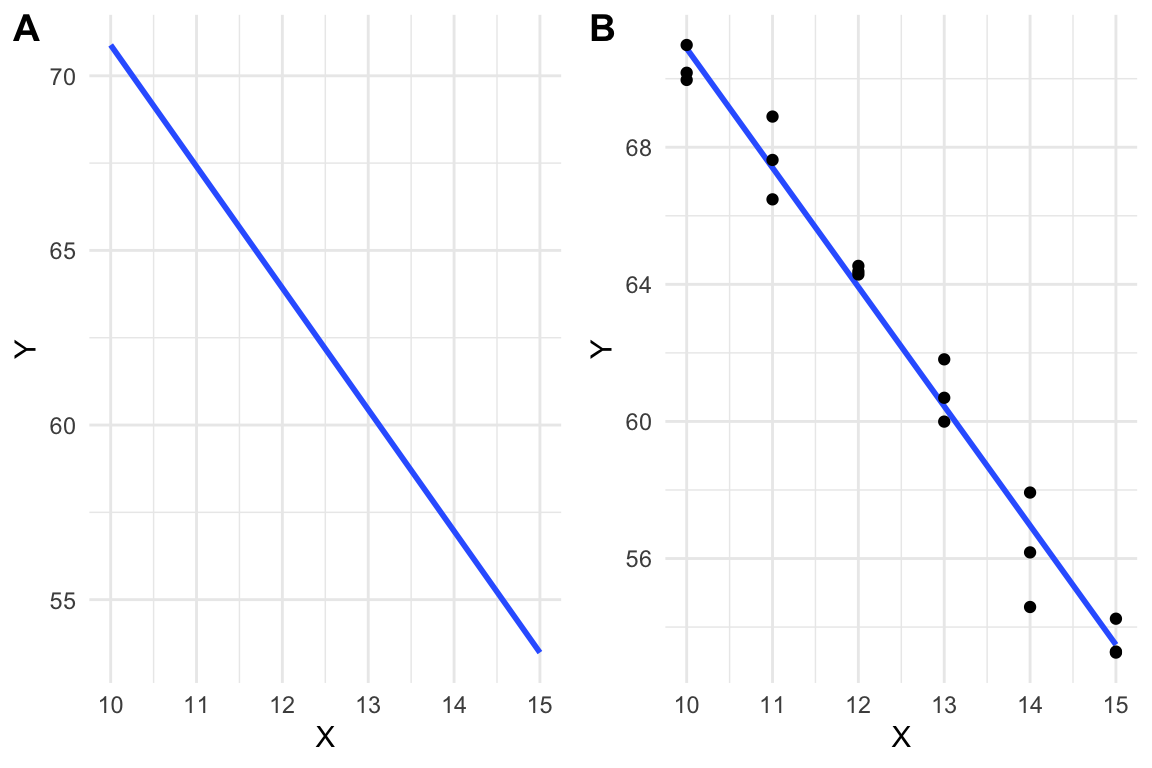
Figure 6.2: A line vs. a linear model. (A) the line \(y=-3.48X + 105.7\) is drawn. (B) A linear model fit to the data. The model coefficients are numerically equal to the slope and intercept of the line in A.
6.3 Two specifications of a linear model
6.3.1 The “error draw” specification
A linear model is commonly specified using
\[\begin{align} Y &= \beta_0 + \beta_1 X + \varepsilon\\ \tag{6.2} \end{align}\]
This specification of a linear model has two parts: the linear predictor \(Y = \beta_0 + \beta_1 X\) and the error \(\varepsilon\). The linear predictor part looks like the equation for a line except that 1) \(\beta_0\) is used for the intercept and \(\beta_1\) for the slope and 2) the intercept term precedes the slope term. This re-labeling and re-arrangement make the notation for a linear model more flexible for more complicated linear models. For example \(Y = \beta_0 + \beta_1 X_1 + \beta_2 X_2 + \varepsilon\) is a model where \(Y\) is a function of two \(X\) variables.
As with the equation for a line, the linear predictor part of a linear model is a function that maps a specific value of \(X\) to a value of \(Y\). This mapped value is the expected value, or expectation, given a specific input value of \(X\). This is often written as \(\mathrm{E}[Y|X]\), which is read as “the expected value of \(Y\) given \(X\)”, where “given X” means a specific value of X. This text will often use the word conditional in place of “given”. It is important to recognize that \(\mathrm{E}[Y|X]\) is a conditional mean – it is the mean value of \(Y\) when we observe that \(X\) has some specific value \(x\).
Introductory textbooks almost always introduce linear models using equation (6.2) above. The key part of the model that is missing from the specification above is a second line \[\begin{equation} \varepsilon \sim N(0, \sigma^2) \end{equation}\]
which is read as “epsilon is distributed as Normal with mean zero and variance sigma squared”. This line explicitly specifies the distribution of the error part. The error part of a linear model is a random “draw” from a normal distribution with mean zero and variance \(\sigma^2\). Using the error-draw specification, we can think of any measurement of \(Y\) as an expected value plus some random value sampled from a specific distribution.
6.3.2 The “conditional draw” specification
A second way of specifying a linear model is
\[\begin{align} y_i &\sim N(\mu_i, \sigma^2)\\ \mathrm{E}(Y|X) &= \mu\\ \mu_i &= \beta_0 + \beta_1 x_i \tag{6.3} \end{align}\]
The first line states that the response variable \(Y\) is a random variable independently drawn from a normal distribution with mean \(\mu\) and variance \(\sigma^2\). This first line is the stochastic part of the statistical model. The second line simply states that \(\mu\) (the greek letter “mu”) from the first line is the conditional mean or conditional expectation. The third line states how \(\mu_i\) is generated given that \(X=x_i\). This is the linear predictor, which is the systematic (or deterministic) part of the statistical model. It is systematic because the same value of \(x_i\) will always generate the same \(\mu_i\).
6.3.3 Comparing the two ways of specifying the linear model
These two ways of specifying the model encourage slightly different ways of thinking about how the data (the response varible \(Y\)) were generated. The error-draw specification “generates” data by 1) constructing what \(y_i\) “should be” given \(x_i\) (this is the conditional expection), then 2) adding some error \(e_i\) drawn from a normal distribution with mean zero and some specified variance. The conditional-draw specification “generates” data by 1) constructing what \(y_i\) “should be” given \(x_i\), then 2) drawing a random variable from some specified distribution whose mean is this expectation. This random draw is not “error” but the measured value \(y_i\). For the error draw generation, we need only one hat of random numbers, but for the conditional draw generation, we need a hat for each value of \(x_i\).
Here is a short script that generates data by implementing both the error-draw and condition-draw specifications.
n <- 5
b_0 <- 10.0
b_1 <- 1.2
sigma <- 0.4
x <- 1:n
y_expected <- b_0 + b_1*x

# error-draw. Note that the n draws are all from the same distribution
set.seed(1)
y_error_draw <- y_expected + rnorm(n, mean = 0, sd = sigma)

# conditional-draw. Note that the n draws are each from a different
# distribution because each has a different mean.
set.seed(1)
y_conditional_draw <- rnorm(n, mean = y_expected, sd = sigma)

data.table(X = x,
           "Y (error draw)" = y_error_draw,
           "Y (conditional draw)" = y_conditional_draw)
## X Y (error draw) Y (conditional draw)
## 1: 1 10.94942 10.94942
## 2: 2 12.47346 12.47346
## 3: 3 13.26575 13.26575
## 4: 4 15.43811 15.43811
## 5: 5 16.13180 16.13180The error-draw specification is not useful for thinking about data generation for data analyzed by generalized linear models, which are models that allow one to specify distribution families other than Normal (such as the binomial, Poisson, and Gamma families). In fact, thinking about a model as a predictor plus error can lead to the misconception that in a generalized linear model, the error (or residuals from the fit) has a distribution from the non-Normal distribution modeled. This cannot be true because the distributions modeled using generalized linear models (other than the Normal) do not have negative values (some residuals must have negative values since the mean of the residuals is zero). Introductory biostatistics textbooks typically only introduce the error-draw specification because introductory textbooks recommend data transformation or non-parametric tests if the data are not approximately normal. This is unfortunate because generalized linear models are extremely useful for real biological data.
Although a linear model (or statistical model more generally) is a model of a data-generating process, linear models are not typically used to actually generate any data. Instead, when we use a linear model to understand something about a real dataset, we think of our data as one realization of a process that generates data like ours. A linear model is a model of that process. That said, it is incredibly useful to use linear models to create fake datasets for at least two reasons: to probe our understanding of statistical modeling generally and, more specifically, to check that a model actually creates data like that in the real dataset that we are analyzing.
6.4 Statistical models are used for prediction, explanation, and description
Researchers typically use statistical models to understand relationships between one or more \(Y\) variables and one or more \(X\) variables. These relationships include
Descriptive modeling. Sometimes a researcher merely wants to describe the relationship between \(Y\) and a set of \(X\) variables, perhaps to discover patterns. For example, the arrival of a spring migrant bird (\(Y\)) as a function of sex (\(X_1\)) and age (\(X_2\)) might show that males and younger individuals arrive earlier. Importantly, if another \(X\) variable is added to the model (or one dropped), the coefficients, and therefore, the precise description, will change. That is, the interpretation of a coefficient as a descriptor is conditional on the other covariates (\(X\) variables) in the model. In a descriptive model, there is no implication of causal effects and the goal is not prediction. Nevertheless, it is very hard for humans to discuss a descriptive model without using causal language, which probably means that it is hard for us to think of these models as mere description. Like natural history, descriptive models are useful as patterns in want of an explanation, using more explicit causal models including experiments.
Predictive modeling. Predictive modeling is very common in applied research. For example, fisheries researchers might model the relationship between population density and habitat variables to predict which subset of ponds in a region are most suitable for brook trout (Salvelinus fontinalis) reintroduction. The goal is to build a model with minimal prediction error, which is the error between predicted and actual values for a future sample. In predictive modeling, the \(X\) (“predictor”) variables are largely instrumental – how these are related to \(Y\) is not a goal of the modeling, although sometimes an investigator may be interested in the relative importance among the \(X\) for predicting \(Y\) (for example, collecting the data may be time consuming, or expensive, or enviromentally destructive, so know which subset of \(X\) are most important for predicting \(Y\) is a useful strategy).
Explanatory (causal) modeling. Very often, researchers are explicitly interested in how the \(X\) variables are causally related to \(Y\). The fisheries researchers that want to reintroduce trout may want to develop and manage a set of ponds to maintain healthy trout populations. This active management requires intervention to change habitat traits in a direction, and with a magnitude, to cause the desired response. This model is predictive – a specific change in \(X\) predicts a specific response in \(Y\) – because the coefficients of the model provide knowledge on how the system functions – how changes in the inputs cause change in the output. Causal interpretation of model coefficients requires a set of strong assumptions about the \(X\) variables in the model. These assumptions are typically met in experimental designs but not observational designs.
With observational designs, biologists are often not very explicit about which of these is the goal of the modeling and use a combination of descriptive, predictive, and causal language to describe and discuss results. Many papers read as if the researchers intend explanatory inference but because of norms within the biology community, mask this intention with “predictive” language. Here, I advocate embracing explicit, explanatory modeling by being very transparent about the model’s goal and assumptions.
6.5 What do we call the \(X\) and \(Y\) variables?
The inputs to a linear model (the \(X\) variables) have many names. In this text, the \(X\) variables are typically * treatment variables – this term makes sense only for variables that are a factor containing the treatment assignment (for example “control” and “treated”) * covariates – this term is usually used for the non-focal \(X\) variables in a statistical model.
A linear model is a regression model and in regression modeling, the \(X\) variables are typically called
- independent variables (often shortened to IV) – “independent” in the sense that in a statistical model at least, the \(X\) are not a function of \(Y\).
- predictor variables (or simply, “predictors”) – this makes the most sense in prediction models.
- explanatory variables – this makes sense in causal models and is usually applied in observational designs.
In this text, the output of a linear model (the \(Y\) variable or variables if the model is multivariate) will most often be calle either of
- response variable (or simply, “response”)
- outcome variable (or simply, “outcome”)
These terms have a causal connotation in everyday english. These terms are often used in regression modeling with observational data, even if the model is not explicitly causal. On other term, common in introductory textbooks, is
- dependent variable – “dependent” in the sense that in a statistical model at least, the \(Y\) is a function of the \(X\).
6.6 Modeling strategy
- exploratory plots is not data mining, or exploring the data for patterns to test. Instead, initial plots are used to
- examine individual points and identify outliers that are likely due to data transcription errors or measurement blunders (not simply odd, but biologically plausible measures).
- provide useful information for initial model filtering (narrowing the list of potential models that are relevant to the question and data). Statistical modeling includes a diverse array of models, yet almost all methods used by researchers in biology, and all models in this book, are generalizations of the linear model specified in (6.3). For some experiments, there may be multiple models that are relevant to the question and data. Model checking (step 3) can help decide which model to ultimately use.
- fit the model, in order to estimate the model parameters and the uncertainty in these estimates.
- check the model, which means to use a series of diagnostic plots and computations of model output to check that the fit model reasonably approximates the data.
- inference from the model, which means to use the fit parameters to learn, with uncertainty, about the system, or to predict future observations, with uncertainty.
- plot the model, which means to plot the data, which may be adjusted, and the estimated parameters (or other results dervived from the estimates) with their uncertainty.
6.7 Fitting the model
If we fit the model
\[\begin{align} Y &= \beta_0 + \beta_1 X + \varepsilon\\ \varepsilon &\sim N(0, \sigma^2) \end{align}\]
we get coefficients that estimate the \(\beta\) parameters, residuals that estimate \(\varepsilon\), and model error that estimates \(\sigma\). The coefficients and residuals can be used to recover the data
\[\begin{equation} y_i = b_0 + b_1 x_i + e_i \end{equation}\]
The coefficients without the residuals are used to calculate the expected values. For experiments where the focus is on the effect of a treatment on some resopnse, these expected values are the same for all the members of a treatment group and this value is the estimated marginal mean of the group. For a prediction model, these expected values are the predicted values or simply, prediction, which is often denoted \(\hat{y}\).
\[\begin{equation} \hat{y}_i = b_0 + b_1 x_i \end{equation}\]
where \(i\) stands for (or “indexes”) the ith case or individual.
If our goal is inference – to infer something about the “population” from the sample using the fit model, then \(\hat{y}_i\) is the point estimate of the parameter \(\mu_i\) (the true mean conditional on \(X\)), the coefficients \(b_0\) and \(b_1\) are point estimates of the parameters \(\beta_0\) and \(\beta_1\), and the standard deviation of the \(e_i\) is an estimate of \(\sigma\). “Population” is in quotes because it is a very abstract concept. Throughout this book, Greek letters refer to a theoretical parameter and Roman letters refer to point estimates.
Throughout this text, I recommend reporting and interpreting interval estimates of the point estimate. A confidence interval is a type of interval estimate. A confidence interval of a parameter is a measure of the uncertainty in the estimate. A 95% confidence interval has a 95% probability (in the sense of long-run frequency) of containing the parameter This probability is a property of the population of intervals that could be computed using the same sampling and measuring procedure. It is not correct, without further assumptions, to state that there is a 95% probability that the parameter lies within the interval. Perhaps a more useful interpretation is that the interval is a compatability interval in that it contains the range of estimates that are compatible with the data, in the sense that a \(t\)-test would not reject the null hypothesis of a difference between the estimate and any value within the interval (this interpretation does not imply anything about the true value).
6.8 Models fit to data in which the \(X\) are treatment variables are regression models
For the model fit to the data in Figure 6.2B, the coefficient of \(X\) is the slope of the line. Perhaps surprisingly, we can fit a model like equation (6.2) to data in which the \(X\) variable is categorical. An example is the ASK1 deletion experiment above (Figure 6.1B). The trick to using a linear model with categorical \(X\) (factor variables) is to recode the factor levels into numbers – how this is done is explained in the chapter on Models with a single Categorical X. When the \(X\) variable is categorical, the coefficients are differences in group means. The linear model fit to the ask1 data has three coefficients (difference in means), one for the effect of HFD alone, one for the effect of the ASK1 knockout (ASK1Δadipo) alone, and one for the interaction effect of HFD and ASK1 knockout.
6.9 Assumptions for inference with a statistical model
Inference refers to using the fit model to generalize from the sample to the population, which assumes that the response is drawn from some specified probability distribution (Normal, or Poisson, or Bernouli, etc.). Throughout this text, I emphasize reporting and interpreting point estimates and confidence intervals. Another kind of inference is a significance test, which is the computation of the probability of “seeing the data” or something more extreme than the data, given a specified null hypothesis. A significance test results in a p-value, which can be reported with the point estimate and confidence interval. Somewhat related to a significance test is a hypothesis test, or a Null-Hypothesis Signficance Test (NHST), in which the \(p\)-value from a significance test is compared to a pre-specified error rate called \(\alpha\). Hypothesis testing was developed as a formal means of decision making but this is rarely the use of NHST in modern biology. For almost all applications of p-values that I see in the literature that I read in ecology, evolution, phyiology, and wet-bench biology, comparing a \(p\)-value to \(\alpha\) adds no value.
- The data were generated by a process that is “linear in the parameters”, which means that the different components of the model are added together. This additive part of the model containing the parameters is the linear predictor in specifications (6.2) and (6.3) above. For example, a cubic polynomial model
\[\begin{equation} \mathrm{E}(Y|X) = \beta_0 + \beta_1 X + \beta_2 X^2 + \beta_3 X^3 \end{equation}\]
is a linear model, even though the function is non-linear, because the different components are added. Because a linear predictor is additive, it can be compactly defined using matrix algebra
\[\begin{equation} \mathrm{E}(Y|X) = \mathbf{X}\boldsymbol{\beta} \end{equation}\]
where \(mathbf{X}\) is the model matrix and \(\boldsymbol{\beta}\) is the vector of parameters. We discuss these more in chapter xxx.
A Generalized Linear Model (GLM) has the form \(g(\mu_i) = \eta_i\) where \(\eta\) (the Greek letter “eta”) is the linear predictor
\[\begin{equation} \eta = \mathbf{X}\boldsymbol{\beta} \end{equation}\]
GLMs are extensions of linear models. There are non-linear models that are not linear in the parameters, that is, the predictor is not a simple dot product of the model matrix and a vector of parameters. For example, the Michaelis-Menten model is a non-linear model
\[\begin{equation} \mathrm{E}(Y|X) = \frac{\beta_1 X}{\beta_2 + X} \end{equation}\]
that is non-linear in the parameters because the parts are not added together. This text covers linear models and generalized linear models, but not non-linear models that are also non-linear in the parameters.
- The draws from the probability distribution are independent. Independence implies uncorrelated \(Y\) conditional on the \(X\), that is, for any two \(Y\) with the same value of \(X\), we cannot predict the value of one given the value of the other. For example, in the ASK1 data above, “uncorrelated” implies that we cannot predict the glucose level of one mouse within a specific treatment combination given the glucose level of another mouse in that combination. For linear models, this assumption is often stated as “independent errors” (the \(\varepsilon\) in model (6.2)) instead of independent observations.
There are lots of reasons that conditional responses might be correlated. In the mouse example, correlation within treatment group could arise if subsets of mice in a treatment group are siblings or are housed in the same cage. More generally, if there are measures both within and among experimental units (field sites or humans or rats) then we’d expect the measures within the same unit to err from the model in the same direction. Multiple measures within experimental units (a site or individual) creates “clustered” observations. Lack of independence or clustered observations can be modeled using models with random effects. These models go by many names including linear mixed models (common in Ecology), hierarchical models, multilevel models, and random effects models. A linear mixed model is a variation of model (6.2). This text introduces linear mixed models in chapter xxx.
Measures that are taken from sites that are closer together or measures taken closer in time or measures from more closely related biological species will tend to have more similar values than measures taken from sites that are further apart or from times that are further apart or from species that are less closely related. Space and time and phylogeny create spatial and temporal and phylogenetic autocorrelation. Correlated error due to space or time or phylogeny can be modeled with Generalized Least Squares (GLS) models. A GLS model is a variation of model (6.2).
6.10 Specific assumptions for inference with a linear model
- Constant variance or homoskedasticity. The most common way of thinking about this is the error term \(\varepsilon\) has constant variance, which is a short way of saying that random draws of \(\varepsilon\) in model (6.2) are all from the same (or identical) distribution. This is explicitly stated in the second line of model specification (6.2). If we were to think about this using model specification (6.3), then homoskedasticity means that \(\sigma\) in \(N(\mu, \sigma)\) is constant for all observations (or that the conditional probability distributions are identical, where conditional would mean adjusted for \(\mu\))
Many biological processes generate data in which the error is a function of the mean. For example, measures of biological variables that grow, such as lengths of body parts or population size, have variances that “grow” with the mean. Or, measures of counts, such as the number of cells damaged by toxin, the number of eggs in a nest, or the number of mRNA transcripts per cell have variances that are a function of the mean. Heteroskedastic error can be modeled with Generalized Least Squares, a generalization of the linear model, and with Generalized Linear Models (GLM), which are “extensions” of the classical linear model.
- Normal or Gaussian probability distribution. As above, the most common way of thinking about this is the error term \(\varepsilon\) is Normal. Using model specification (6.3), we’d say the conditional probablity distribution of the response is normal. A normal probability distribution implies that 1) the response is continuous and 2) the conditional probability is symmetric around \(mu_i\). If the conditional probability distribution has a long left or right tail it is skewed left or right. Counts (number of cells, number of eggs, number of mRNA transcripts) and binary responses (sucessful escape or sucessful infestation of host) are not continuous and often often have asymmetric probablity distributions that are skewed to the right and while sometimes both can be reasonably modeled using a linear model they are more often modeled using generalized linear models, which, again, is an extension of the linear model in equation (6.3). A classical linear model is a specific case of a GLM.
A common misconception is that inference from a linear model assumes that the unconditional response (this is just the response variable) is normally distributed. Both the error-draw and conditional-draw specifications of a linear model show precisely why this conception is wrong. Model (6.2) states explicitly that it is the error that has the normal distribution – the distribution of \(Y\) is a mix of the distribution of \(X\) and the error. Model (6.3) states that the conditional outcome has a normal distribution, that is, the distribution after adjusting for variation in \(X\).
6.11 “linear model,”regression model“, or”statistical model"?
Statistical modeling terminology can be confusing. The \(X\) variables in a statistical model may be quantitative (continuous or integers) or categorical (names or qualitative amounts) or some mix of the two. Linear models with all quantitative independent variables are often called “regression models.” Linear models with all categorical independent variables are often called “ANOVA models.” Linear models with a mix of quantitative and categorical variables are often called “ANCOVA models” if the focus is on one of the categorical \(X\) or “regression models” if there tend to be many independent variables.
This confusion partly results from the history of the development of regression for the analysis of observational data and ANOVA for the analysis of experimental data. The math underneath classical regression (without categorical variables) is the linear model. The math underneath classical ANOVA is the computation of sums of squared deviations from a group mean, or “sums of squares”. The basic output from a regression is a table of coefficients with standard errors. The basic ouput from ANOVA is an ANOVA table, containing the sums of squares along with mean-squares, F-ratios, and p-values. Because of these historical differences in usage, underlying math, and output, many textbooks in biostatistics are organized around regression “vs.” ANOVA, presenting regression as if it is “for” observational studies and ANOVA as if it is “for” experiments.
It has been recognized for many decades that experiments can be analyzed using the technique of classical regression if the categorical variables are coded as numbers (again, this will be explained later) and that both regression and ANOVA are variations of a more general, linear model. Despite this, the “regression vs. ANOVA” way-of-thinking dominates the teaching of biostatistics.
To avoid misconceptions that arise from thinking of statistical analysis as “regression vs. ANOVA”, I will use the term “linear model” as the general, umbrella term to cover everything in this book. By linear model, I mean any model that is linear in the parameters, including classical regression models, marginal models, linear mixed models, and generalized linear models. To avoid repetition, I’ll also use “statistical model”.