Chapter 13 Best practices – issues in inference
13.1 Multiple testing
Multiple testing is the practice of adjusting p-values (and less commonly confidence intervals) to account for the expected increase in the frequency of Type I error when there are multiple tests (typically Null Hypothesis Significance Tests). Multiple testing tends to arise in two types of situations:
- Multiple pairwise contrasts among treatment levels (or combinations of levels) are estimated.
- The effects of a treatment on multiple responses are estimated. This can arise if
- there are multiple ways of measuring the consequences of something – for example, an injurious treatment on plant health might effect root biomass, shoot biomass, leaf number, leaf area, etc.
- one is exploring the consequences of an effect on many, many outcomes – for example, the expression levels of 10,000 genes between normal and obese mice.
Despite the ubiquitous presence of multiple testing in elementary biostatistics textbooks, in the applied biology literature, and in journal guidelines, the practice of adjusting p-values for multiple tests is highly controversial among statisticians. My thoughts:
- In situations like (1) above, I advocate that researchers do not adjust p-values for multiple tests. In general, its a best practice to only estimate contrasts for which you care about because of some a priori model of how the system works. If you compare all pairwise contrasts of an experiment with many treatment levels and/or combinations, expect to find some false discoveries.
- In situations like (2a) above, I advocate that researchers do not adjust p-values for multiple tests.
- In situations like (2b) above, adjusting for the False Discovery Rate is an interesting approach. But, recognize that tests with small p-values are highly provisional discoveries of a patterns only and not a discovery of the causal sequelae of the treatment. For that, one needs to do the hard work of designing experiments that rigorously probe a working, mechanistic model of the system.
Finally, recognize that anytime there are multiple tests, Type M errors will arise due to the vagaries of sampling. This means that in a rank-ordered list of the effects, those at the top have measured effects that are probably bigger than the true effect. An alternative to adjusted p-values is a penalized regression model that shrinks effects toward the mean effect.
13.1.1 Some background
13.1.1.1 Family-wise error rate
The logic of multiple testing goes something like this: the more tests that a researcher does, the higher the probability that a false positive (Type I error) will occur, therefore a researcher should should adjust p-values so that the Type I error over the set (or “family”) of tests is 5%. This adjusted Type I error rate is the “family-wise error rate”.
If a researcher carries out multiple tests of data in which the null hypothesis is true, what is the probability of finding at least one Type I error? This is easy to compute. If the frequency of Type I error for a single test is , then the probability of no Type I error is . For two tests, the probability of no Type I error in either test is the product of the probability for each test, or . By the same logic, for tests, the probabilty of no type I error in any of the tests is . The probability of at least one type one error, across the tests, then, is . A table of these probabilities for different is given below. If the null is true in all tests, then at least one Type I error is more likely than not if there are 14 tests, and close to certain if there more than 50 tests. Don’t skip over this paragraph – the logic is important even if I don’t advocate adjusting for multiple tests.
| m | p |
|---|---|
| 1 | 0.05 |
| 3 | 0.14 |
| 6 | 0.26 |
| 10 | 0.40 |
| 50 | 0.92 |
| 100 | 0.99 |
13.1.1.2 False discovery rate
If a researcher carries out thousands of tests to “discover” new facts, and uses as evidence of discovery, then what is the frequency of false discoveries?
13.1.1.3 p-value filter I – Inflated effects
If a researcher caries out many tests, and ranks the effects by magnitude or p-value, then the effect sizes of the largest effects will be inflated. Before explaining why, let’s simulate this using an experiment of allelopathic effects of the invasive garlic mustard (Alliaria petiolata) on gene expression in the native American ginseng (Panax quinquefolius). In the treated group, we have ten pots, each with an American ginseng plant grown in a container with a mustard plant. In the control group, we have ten pots, each with an American ginseng plant grown in a container with another American ginseng. I’ve simulated the response of 10,000 genes. The treatment has a true effect in 10% of the 10,000 genes but most effects are very small.
set.seed(4)
p <- 10^4 # number of genes
pt <- 0.1*p # number of genes with true response to treatment
n <- 10

# sample the gene effects from an exponential distribution
theta <- .3
beta <- c(rexp(pt, rate=1/theta),
          rep(0, (p-pt))) # the set of 10,000 effects

# sample the variance of the expression level with a gamma, and set a minimum
sigma <- rgamma(p, shape=2, scale=1/4) + 0.58
# quantile(sigma, c(0.001, 0.1, 0.5, 0.9, 0.999))

Y1 <- matrix(rnorm(n*p, mean=0, sd=rep(sigma, each=n)), nrow=n)
Y2 <- matrix(rnorm(n*p, mean=rep(beta, each=n), sd=rep(sigma, each=n)), nrow=n) # check
# use n <- 10^4 to check
# apply(y2, 2, mean)[1:5]
# b[1:5]
x <- rep(c("cn","tr"), each=n)
bhat <- numeric(p)
p.value <- numeric(p)
sigma_hat <- numeric(p)
for(j in 1:p){
  fit <- lm(c(Y1[,j], Y2[, j]) ~ x)
  bhat[j] <- coef(summary(fit))["xtr", "Estimate"]
  p.value[j] <- coef(summary(fit))["xtr", "Pr(>|t|)"]
  sigma_hat[j] <- sqrt(sum(fit$residuals^2)/fit$df.residual)
}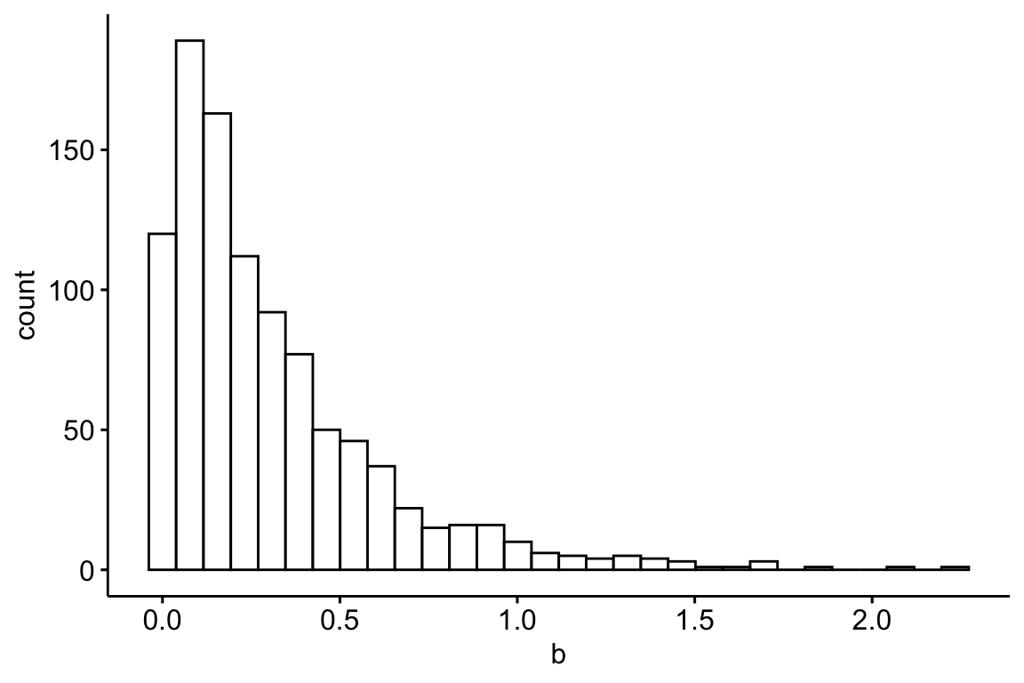
Figure 13.1: A histogram of the distribution of the 10,000 effects
| effect | estimate | sigma | sd | p.value | relative true effect | rank |
|---|---|---|---|---|---|---|
| 2.23 | 2.67 | 0.81 | 0.55 | 0.0000000 | 1.00 | 1 |
| 1.59 | 1.92 | 0.62 | 0.57 | 0.0000005 | 0.71 | 7 |
| 1.46 | 1.86 | 0.84 | 0.71 | 0.0000159 | 0.65 | 10 |
| 1.47 | 1.78 | 0.83 | 0.74 | 0.0000409 | 0.66 | 9 |
| 0.00 | 1.95 | 1.10 | 0.85 | 0.0000717 | 0.00 | NA |
| 0.48 | 1.26 | 0.67 | 0.56 | 0.0000816 | 0.21 | 212 |
| 0.97 | 1.32 | 0.69 | 0.60 | 0.0001004 | 0.43 | 45 |
| 0.54 | 1.68 | 1.06 | 0.78 | 0.0001321 | 0.24 | 173 |
| 0.00 | 2.05 | 1.39 | 0.96 | 0.0001488 | 0.00 | NA |
| 0.43 | -1.78 | 1.33 | 0.84 | 0.0001733 | 0.19 | 244 |
The table above lists the top 10 genes ranked by p-value, using the logic that the genes with the smallest p values are the genes that we should pursue with further experiments to understand the system. Some points
- Six of the top ten genes with biggest true effects are not on this list. And, in the list are three genes with true effects that have relatively low ranks based on true effect size (column "rank") and two genes that have no true effect at all. Also in this list is one gene with an estimated effect (-1.78) that is opposite in sign of the true effect (but look at the p-value!)
- The estimate of the effect size for all top-ten genes are inflated. The average estimate for these 10 genes is 1.47 while the average true effect for these 10 genes is 0.92 (the estimate ).
- The sample standard deviation (sd) for all top-ten genes is less than the true standard deviation (sigma), in some cases substantially.
The consequence of an inflated estimate of the effect and a deflated estimate of the variance is a large t (not shown) and small p. What is going on is an individual gene’s estimated effect and standard deviation are functions of 1) the true value and 2) a random sampling component. The random component will be symmetric, some effects will be overestimated and some underestimated. When we rank the genes by the estimate of the effect or t or p, some of the genes that have “risen to the top” will be there because of a large, positive, sampling (random) component of the effect and/or a large, negative, sampling component of the variance. Thus some genes’ high rank is artificial in the sense that it is high because of a random fluke. If the experiment were re-done, these genes at the top because of a large, random component would (probably) fall back to a position closer to their expected rank (regression to the mean again).
In the example here, all genes at the top have inflated estimates of the effect because of the positive, random component. This inflation effect is a function of the signal to noise ratio, which is controled by theta and sigma in the simulation. If theta is increased (try theta=1), or if sigma is decreased, the signal to noise ratio increases (try it and look at the histogram of the new distribution of effects) and both the 1) inflation and the 2) rise to the top phenomenon decrease.
13.1.1.4 p-hacking
13.1.2 Multiple testing – working in R
13.1.2.1 Tukey HSD adjustment of all pairwise comparisons
The adjust argument in emmeans::contrast() controls the method for p-value adjustment. The default is “tukey”.
- “none” – no adjustment, in general my preference.
- “tukey” – Tukey’s HSD, the default
- “bonferroni” – the standard bonferroni, which is conservative
- “fdr” – the false discovery rate
- “mvt” – based on the multivariate t distribution and using covariance structure of the variables
The data are those from Fig. 2D of “Data from The enteric nervous system promotes intestinal health by constraining microbiota composition”. There is a single factor with four treatment levels. The response is neutrophil count.
No adjustment:
m1 <- lm(count ~ donor, data=exp2d)
m1.emm <- emmeans(m1, specs="donor")
m1.pairs.none <- contrast(m1.emm, method="revpairwise", adjust="none")
summary(m1.pairs.none, infer=c(TRUE, TRUE))
## contrast estimate SE df lower.CL upper.CL t.ratio p.value
## gf - wt -1.502 1.48 58 -4.47 1.47 -1.013 0.3153
## sox10 - wt 4.679 1.23 58 2.23 7.13 3.817 0.0003
## sox10 - gf 6.182 1.45 58 3.29 9.08 4.276 0.0001
## iap_mo - wt -0.384 1.53 58 -3.45 2.68 -0.251 0.8025
## iap_mo - gf 1.118 1.71 58 -2.31 4.54 0.654 0.5159
## iap_mo - sox10 -5.064 1.49 58 -8.05 -2.07 -3.391 0.0013
##
## Confidence level used: 0.95Tukey HSD:
m1.pairs.tukey <- contrast(m1.emm, method="revpairwise", adjust="tukey")
summary(m1.pairs.tukey, infer=c(TRUE, TRUE))
## contrast estimate SE df lower.CL upper.CL t.ratio p.value
## gf - wt -1.502 1.48 58 -5.43 2.42 -1.013 0.7426
## sox10 - wt 4.679 1.23 58 1.44 7.92 3.817 0.0018
## sox10 - gf 6.182 1.45 58 2.36 10.01 4.276 0.0004
## iap_mo - wt -0.384 1.53 58 -4.43 3.66 -0.251 0.9944
## iap_mo - gf 1.118 1.71 58 -3.41 5.64 0.654 0.9138
## iap_mo - sox10 -5.064 1.49 58 -9.01 -1.11 -3.391 0.0067
##
## Confidence level used: 0.95
## Conf-level adjustment: tukey method for comparing a family of 4 estimates
## P value adjustment: tukey method for comparing a family of 4 estimates13.1.3 False Discovery Rate
13.2 difference in p is not different
13.3 Inference when data are not Normal
No real data are normal, although many are pretty good approximations of a normal distribution.
I’ll come back to this point, but first, let’s back up. Inference in statistical models (standard errors, confidence intervals, p-values) are a function of the modeled distributions of the parameters (for linear models, this parameter is the conditional (or error) variance ); if the data do not approximate the modeled distribution, then inferential statistics might be to liberal (standard errors are too small, confidence intervals are too narrow, Type I error is more than nominal) or to conservative (standard errors are too large, confidence intervals are too wide, Type I error is less than nominal).
Linear models assume that “the data” (specifically, the conditional response, or, equivalently, the residuals from the model) approximate a Normal distribution. Chapter xxx showed how to qualitatively assess how well residuals approximate a Normal distribution using a Q-Q plot. If the researcher concludes that the data poorly approximate a normal distribution because of outliers, the researcher can use robust methods to estimate the parameters. If the approximation is poor because the residuals suggest a skewed distribution or one with heavy or light tails, the researcher can choose among several strategies
- continue to use the linear model; inference can be fairly robust to non-normal data, especially when the sample size is not small.
- use a generalized linear model (GLM), which is appropriate if the conditional response approximates any of the distributions that can be modeled using GLM (Chapter xxx)
- use bootstrap for confidence intervals and permutation test for p-values
- transform the data in a way that makes the conditional response more closely approximate a normal distribution.
- use a classic non-parametric test, which are methods that do not assume a particular distribution
This list is roughly in the order of how I would advise researchers, although the order of 1-3 is pretty arbitrary. I would rarely advise a researcher to use (4) and never advise (5). Probably the most common strategies in the biology literature are (4) and (5). The first is also common but probably more from lack of recognition of issues or because a “test of normality” failed to reject that the data are “not normal”.
On this last point, do not use the p-value from a “test for normality” (such as a Shapiro-Wilk test) to decide between using the linear model (or t-test or ANOVA) and an alternative such as a generalized linear model (or transformation or non-parametric test). No real data is normal. Tests of normality will tend to “not reject” normality (p > 0.05) when the sample size is small and “reject” normality (p < 0.05) when the sample size is very large. But again, a “not rejected” hypothesis test does not mean the null (in this case, the data are normal) is true. More importantly, where the test for normality tends to fail to reject (encouraging a researcher to use parametric statistics) is where parametric inference performs the worst (because of small n) and where the test for normality tends to reject (encouraging a researcher to use non-parametric statistics) is where the parametric inference performs the best (because of large sample size) (Lumley xxx).
13.3.1 Working in R
The data for demonstrating different strategies are from Fig. 4A of “Data from The enteric nervous system promotes intestinal health by constraining microbiota composition”. There is a single factor with two treatment levels. The response is neutrophil count.
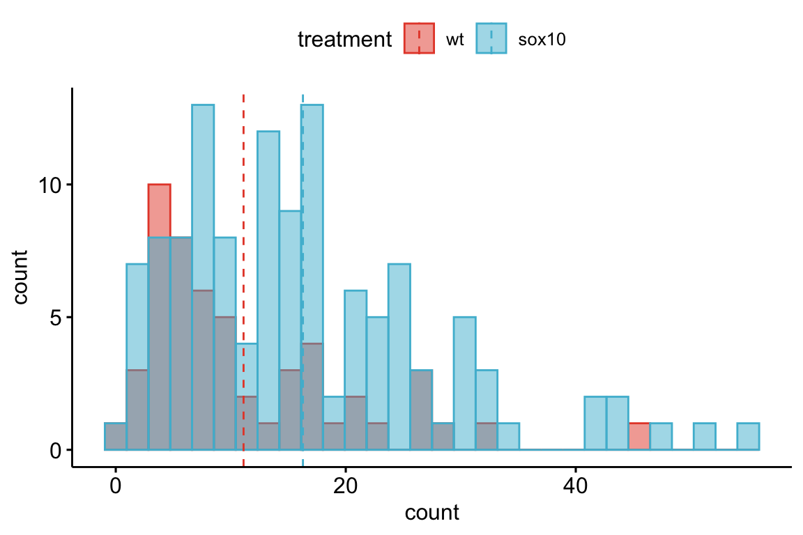
Figure 13.2: Distribution of the counts in the wildtype (WT) and sox10 knockout (sox10-) groups. Both groups show a strong right skew, which is common with count data.
A linear model to estimate the treatment effect and 95% confidence interval.
m1 <- lm(count ~ treatment, data=fig4a)
m1_emm <- emmeans(m1, specs="treatment")
summary(contrast(m1_emm, method="revpairwise"),
        infer=c(TRUE, TRUE))
## contrast estimate SE df lower.CL upper.CL t.ratio p.value
## sox10 - wt 5.16 1.75 174 1.7 8.62 2.947 0.0037
##
## Confidence level used: 0.9513.3.2 Bootstrap Confidence Intervals
A bootstrap confidence interval is computed from the distribution of a statistic from many sets of re-sampled data. The basic algorithm is
- compute the statistic for the observed data, assign this to
- resample rows of the data, with replacement. “with replacement” means to sample from the entire set of data and not the set that has yet to be sampled. is the original sample size; by resampling rows with replacement, some rows will be sampled more than once, and some rows will not be sampled at all.
- compute the statistic for the resampled data, assign these to
- repeat 2 and 3 times
- Given the distribution of estimates, compute the lower interval as the th percentile and the upper interval as the th percentile. For 95% confidence intervals, these are the 2.5th and 97.5th percentiles.
Let’s apply this algorithm to the data from fig4A neutrophil count data in the coefficient table above. The focal statistic in these data is the difference in the mean count for the sox10 and wild type groups (the parameter for in the linear model). The script below, which computes the 95% confidence intervals of this difference, resamples within strata, that is, within each group; it does this to preserve the original sample size within each group.
n_iter <- 5000
b1 <- numeric(5000)
inc <- 1:nrow(fig4a) # the rows for the first iteration are all rows, so this is the observed effect
for(i in 1:n_iter){
  # inc creates the index of rows to resample preserving the sample size specific to each group
  b1[i] <- coef(lm(count ~ treatment, data=fig4a[inc, ]))["treatmentsox10"]
  inc <- c(sample(which(fig4a[, treatment] == "wt"), replace=TRUE),
           sample(which(fig4a[, treatment] == "sox10"), replace=TRUE))
}
ci <- quantile(b1, c(0.025, 0.975))
c(contrast = b1[1], ci[1], ci[2])
## contrast 2.5% 97.5%
## 5.163215 2.077892 8.264316The intervals calculated in step 5 are percentile intervals. A histogram of the the re-sampled differences helps to visualize the bootstrap (this is a pedagogical tool, not something you would want to publish).
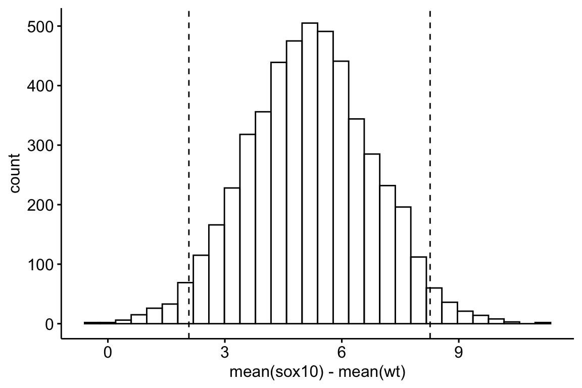
Figure 13.3: Distribution of the 5000 resampled estimates of the difference in means between the sox10 and wt treatment levels. The dashed lines are located at the 2.5th and 97.5th percentiles of the distribution.
13.3.2.1 Some R packages for bootstrap confidence intervals
Percentile intervals are known to be biased, meaning the intervals are shifted. The boot package computes a bias-corrected interval in addition to a percentile interval. boot is a very powerful bootstrap package but requires the researcher to write functions to compute the parameter of interest. simpleboot provides functions for common analysis that does this for you (in R speak, we say that simpleboot is a “wrapper” to boot). The function simpleboot::two.boot computes a boot-like object that returns, among other values, the distribution of statistics. The simpleboot object is then be fed to boot::boot.ci to get bias-corrected intervals.
bs_diff <- two.boot(fig4a[treatment=="sox10", count],
                    fig4a[treatment=="wt", count],
                    mean,
                    R=5000)
boot.ci(bs_diff, type="bca")
## BOOTSTRAP CONFIDENCE INTERVAL CALCULATIONS
## Based on 5000 bootstrap replicates
##
## CALL :
## boot.ci(boot.out = bs_diff, type = "bca")
##
## Intervals :
## Level BCa
## 95% ( 2.087, 8.410 )
## Calculations and Intervals on Original Scale13.3.3 Permutation test
A permutation test effectively computes the probability that a random assignment of a response to a particular value of X generates a test statistic as large or larger than the observed statistic. If this probability is small, then this “random assignment” is unlikely. From this we infer that the actual assignment matters, which implies a treatment effect.
The basic algorithm is
- compute the test statistic for the observed data, assign this to
- permute the response
- compute the test statistic for the permuted data, assign these to
- repeat 2 and 3 times
- compute as
This is easily done with a for loop in which the observed statistic is the first value in the vector of statistics. If this is done, the minimum value in the numerator for the computation of is 1, which insures that is not zero.
The test statistic depends on the analysis. For the simple comparison of means, a simple test statistic is the difference in means. This is the numerator of the test statistic in a t-test. The test has more power if the test-statistic is scaled (Manley xxx), so a better test statistic would be t, which scales the difference by its standard error.
Here, I implement this algorithm. The test is two-tailed, so the absolute difference is recorded. The first value computed is the observed absolute difference.
set.seed(1)
n_permutations <- 5000
d <- numeric(n_permutations)

# create a new column which will contain the permuted response
# for the first iteration, this will be the observed order
fig4a[, count_perm := count]

for(i in 1:n_permutations){
  d[i] <- abs(t.test(count_perm ~ treatment, data = fig4a)$statistic)

  # permute the count_perm column for the next iteration
  fig4a[, count_perm := sample(count)]
}
p <- sum(d >= d[1])/n_permutations
p
## [1] 0.00213.3.3.1 Some R packages with permutation tests.
lmPerm::lmp generates permutation p-values for parameters of any kind of linear model. The test statistic is the sum of squares of the term scaled by the residual sum of squares of the model.
## [1] "Settings: unique SS "## Estimate Iter Pr(Prob)
## (Intercept) 13.694815 5000 0.0042
## treatment1 -2.581608 5000 0.004213.3.4 Non-parametric tests
- In general, the role of a non-parametric test is a better-behaved p-value, that is, one whose Type I error is well controlled. As such, non-parametric tests are more about Null-Hypothesis Statistical Testing and less (or not at all) about Estimation.
- In general, classic non-parametric tests are only available for fairly simple experimental designs. Classic non-parametric tests include
- Independent sample (Student’s) t test: Mann-Whitney-Wilcoxan
- Paired t test: Wilcoxan signed-rank test
One rarely sees non-parametric tests for more complex designs that include covariates, or multiple factors, but for these, one could 1) convert the response to ranks and fit the usual linear model, or 2) implement a permutation test that properly preserves exchangeability.
Permutation tests control Type I error and are powerful. That said, I would recommend a permutation test as a supplment to, and not replacement of, inference from a generalized linear model.
A non-parametric (Mann-Whitney-Wilcoxon) test of the fake data generated above
##
##  Wilcoxon rank sum test with continuity correction
##
## data:  count by treatment
## W = 2275, p-value = 0.001495
## alternative hypothesis: true location shift is not equal to 0
13.3.5 Log transformations
Many response variables within biology, including count data, and almost anything that grows, are right skewed and have variances that increase with the mean. A log transform of a response variable with this kind of distribution will tend to make the residuals more approximately normal and the variance less dependent of the mean. At least two issues arise
- if the response is count data, and the data include counts of zero, then a fudge factor has to be added to the response since log(0) doesn’t exist. The typical fudge factor is to add 1 to all values, but this is arbitrary and results do depend on the magnitude of this fudge factor.
- the estimates are on a log scale and do not have the units of the response. The estimates can be back-transformed by taking the exponent of a coefficient or contrast but this itself produces problems. For example, the backtransformed mean of the log-transformed response is not the mean on the origianl scale (the arithmetic mean) but the geometric mean. Geometric means are smaller than arithmetic means, appreciably so if the data are heavily skewed. Do we want our understanding of a system to be based on geometric means?
13.3.5.1 Working in R – log transformations
If we fit a linear model to a log-transformed response then the resulting coefficients and predictions are on the log scale. To make interpretation of the analysies easier, we probably want to back-transform the coefficients or the predictions to the original scale of the response, which is called the response scale.
m2 <- lm(log(count + 1) ~ treatment, data=fig4a)
(m2_emm <- emmeans(m2,
                  specs="treatment",
                  type = "response"))
## treatment response SE df lower.CL upper.CL
## wt 8.22 0.965 174 6.5 10.3
## sox10 12.59 0.934 174 10.9 14.6
##
## Confidence level used: 0.95
## Intervals are back-transformed from the log(mu + 1) scaleThe emmeans package is amazing. Using the argument type = "response" not only backtransforms the means to the response scale but also substracts the 1 that was added to all values in the model.
What about the effect of treatment on count?
##  contrast   ratio    SE  df lower.CL upper.CL t.ratio p.value
##  sox10 / wt  1.47 0.185 174     1.15     1.89 3.100   0.0023
##
## Confidence level used: 0.95
## Intervals are back-transformed from the log scale
## Tests are performed on the log scale
It isn’t necessary to backtransform the estimated marginal means prior to computing the contrasts as this can be done in the contrast function itself. Here, the type = "response" argument in the contrast function is redundant since this was done in the computation of the means. But it is transparent so I want it there.
Don’t skip this paragraph Look at the value in the “contrast” column – it is “sox10 / wt” and not “sox10 - wt”. The backtransformed effect is a ratio instead of a difference. A difference on the log scale is a ratio on the response scale because of this equality
The interpretation is: If is the backtransformed effect, then, given a one unit increase in , the expected value of the response increases . For a categorical , this means the backtransformed effect is the ratio of backtransformed means – its what you have to multiply the mean of the reference by to get the mean of the treated group. And, because it is the response that is log-transformed, these means are not arithemetic means but geometric means. Here, this is complicated by the model – the response is not a simple log transformation but log(response + 1). It is easy enough to get the geometric mean of the treated group – multiply the backtransformed intercept by the backtransformed coefficient and then subtract 1 – but because of this subtraction of 1, the interpretation of the backtransformed effect is awkward at best (recall that I told you that a linear model of a log transformed response, and especially the log of the response plus one, leads to difficulty in interpreting the effects).
# backtransformed control mean -- a geometric mean
mu_1 <- exp(coef(m2)[1])

# backtransformed effect
b1_star <- exp(coef(m2)[2])

# product minus 1
mu_1*b1_star -1
## (Intercept)
## 12.59357# geometric mean of treatment group
n <- length(fig4a[treatment=="sox10", count])
exp(mean(log(fig4a[treatment=="sox10", count+1])))-1## [1] 12.59357Back-transformed effect
##    (Intercept) treatmentsox10
##       9.219770       1.474394
13.3.6 Performance of parametric tests and alternatives
13.3.6.1 Type I error
If we are going to compute a -value, we want it to be uniformly distributed “under the null”. A simple way to check this is to compute Type I error. If we set , then we’d expect 5% of tests of an experiment with no effect to have .
# first create a matrix with a bunch of data sets, each in its own column
n <- 10
n_sets <- 4000
fake_matrix <- rbind(matrix(rnegbin(n*n_sets, mu=10, theta=1), nrow=n),
                   matrix(rnegbin(n*n_sets, mu=10, theta=1), nrow=n))
treatment <- rep(c("cn", "tr"), each=n)

tests <- c("lm", "log_lm","mww", "perm")
res_matrix <- matrix(NA, nrow=n_sets, ncol=length(tests))
colnames(res_matrix) <- tests
for(j in 1:n_sets){
  res_matrix[j, "lm"] <- coef(summary(lm(fake_matrix[,j] ~ treatment
                                 )))[2, "Pr(>|t|)"]
  res_matrix[j, "log_lm"] <- coef(summary(lm(log(fake_matrix[,j] + 1) ~ treatment
                                 )))[2, "Pr(>|t|)"]
  res_matrix[j, "mww"] <- wilcox.test(fake_matrix[,j] ~ treatment,
                                      exact=FALSE)$p.value
  res_matrix[j, "perm"] <- coef(summary(lmp(fake_matrix[,j] ~ treatment,
                                 perm="Prob", Ca=0.01)))[2, "Pr(Prob)"]
}## lm log_lm mww perm
## 0.04150 0.05250 0.04350 0.04675Type I error is computed for the linear model, the linear model with a log transformed responpse, Mann-Whitney-Wilcoxon, and permutation tests. All four tests are slightly conservative for data that look like that modeled. The computed Type I error of the permutation test is closest to the nominal value of 0.05.
13.3.6.2 Power
Power is the probability of a test to reject the null hypothesis if the null hypothesis is false (that is, if an effect exists)
If all we care about is a then we want to use a test that is most powerful. But, while power is defined using , we can care about power even if we don’t consider to be a very useful concept because increased power also increases the precision of an estimate (that is, narrows confidence intervals).
# first create a matrix with a bunch of data sets, each in its own column
n <- 5
n_sets <- 4000
fake_matrix <- rbind(matrix(rnegbin(n*n_sets, mu=10, theta=1), nrow=n),
                   matrix(rnegbin(n*n_sets, mu=20, theta=1), nrow=n))
treatment <- rep(c("cn", "tr"), each=n)

tests <- c("lm", "log_lm","mww", "perm")
res_matrix <- matrix(NA, nrow=n_sets, ncol=length(tests))
colnames(res_matrix) <- tests
for(j in 1:n_sets){
  res_matrix[j, "lm"] <- coef(summary(lm(fake_matrix[,j] ~ treatment
                                 )))[2, "Pr(>|t|)"]
  res_matrix[j, "log_lm"] <- coef(summary(lm(log(fake_matrix[,j] + 1) ~ treatment
                                 )))[2, "Pr(>|t|)"]
  res_matrix[j, "mww"] <- wilcox.test(fake_matrix[,j] ~ treatment,
                                      exact=FALSE)$p.value
  res_matrix[j, "perm"] <- coef(summary(lmp(fake_matrix[,j] ~ treatment,
                                 perm="Prob", Ca=0.01)))[2, "Pr(Prob)"]
}## lm log_lm mww perm
## 0.09200 0.12525 0.08375 0.10600As above, Power is computed for the linear model, linear model with a log-transformed response, Mann-Whitney-Wilcoxan, and permutation, by simulating a “low power” experiment. The effect is huge (twice as many cells) but the power is low because the sample size is small (). At this sample size, and for this model of fake data, all tests have low power. The power of the log-transformed response is the largest. A problem is, this is not a test of the means but of the log transformed mean plus 1. The power of the permutation test is about 25% larger than that of the linear model and Mann-Whitney-Wilcoxan test. An advantage of this test is that it is a p-value of the mean. A good complement to this p-value would be bootstraped confidence intervals. Repeat this simulation using do see how the relative power among the three change in a simulation of an experiment with more power.